
Managing large spreadsheets is difficult enough without worrying about hidden duplicates skewing your totals and analysis. Manually reviewing thousands of rows is inefficient and prone to human error. Fortunately, Excel provides built-in tools to surface these inconsistencies instantly. In this guide, we will show you how to use Conditional Formatting to highlight duplicate (or unique) values so you can manage your data with confidence.
As datasets grow, even small inconsistencies can quietly undermine accuracy, reporting, and decision‑making. Duplicate entries may not always be obvious at a glance, yet they can distort totals, skew analysis, and create confusion when data is shared across teams. Having a reliable way to surface and address these issues early can save hours of cleanup later and help maintain confidence in the data you rely on every day.
Manually reviewing long columns row by row is not only inefficient, it also increases the risk of human error. When similar values appear scattered throughout a worksheet, duplicates can easily be overlooked or removed inconsistently. This is where built‑in Excel tools become especially valuable, allowing you to identify patterns and problem areas quickly without altering the underlying data structure.
Excel makes that easy by allowing to format the cells using a conditional format which will highlight the duplicate cells so you can remove the duplicates. It can also be used to highlight unique values. Be aware that you cannot conditionally format fields in the Values area of a PivotTable report by unique or duplicate values.
Note: You cannot apply this specific conditional formatting rule to fields in the Values area of a PivotTable report.

How to Highlight Duplicate Cells
1. Select your data: Highlight the range of cells, columns, or rows you want to check for duplicates.
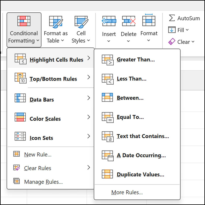
2. Open Conditional Formatting: On the Home tab, look for the Styles group and click Conditional Formatting.
3. Choose the Rule: Hover over Highlight Cells Rules and select Duplicate Values… from the slide-out menu.
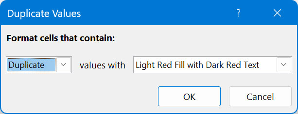
4. Configure the Format: In the pop-up box, ensure “Duplicate” is selected in the first dropdown. In the second dropdown, choose your preferred highlight color (e.g., “Light Red Fill with Dark Red Text”).
5. Click OK: All duplicate entries in your selected range will now be highlighted.
Now all the duplicate cells will be highlighted with the color you chose making it easy to find and remove them.
How to Quickly Remove Duplicates
If you don’t need to see the highlights and just want the duplicates gone:
- Select your data range.
- Go to the Data tab.
- In the Data Tools group, click Remove Duplicates.
- Choose which columns to check and click OK. Excel will tell you exactly how many duplicate values were found and removed.
In summary, Excel’s conditional formatting tools provide a fast, reliable way to identify duplicate and unique values without disrupting your data. By visually flagging potential issues, you can maintain cleaner spreadsheets, reduce errors, and spend less time on manual reviews. This approach not only improves efficiency but also helps ensure that your data remains accurate and trustworthy as your worksheets continue to grow.