As you probably know, Microsoft Excel can do much more than most people ever use it for but that doesn’t mean you shouldn’t try and learn something new because it might come in handy! Then the more you know, the more you will be able to do with Excel in the future.
Since an Excel workbook is capable of holding a lot of data it’s nice to be able to filter that data when needed to make things easier to find and also easier to see. Sure you can use the filtering options on the Data tab but Excel has another way to filter your data that is much cooler and it’s called Slicers.
What Slicers does is take the data you want to view and slice it right out of the sheet so you only see what you want to see. Then you can fine tune these slices to filter things at an even more granular level making it very easy to see only the information you are interested in. Plus once you have your slices setup it’s easy to edit them to change what information you will see in your filtered results.
To use Slicers go to the Filter section on the Insert tab and then go to Filters group. There you will see the Slicers button that you can use to slice out values that you want to filter on. As you can see below we have a spreadsheet with a lot of columns and rows and a ton of information. We need to filter this data so we can see the information we care about at the moment.
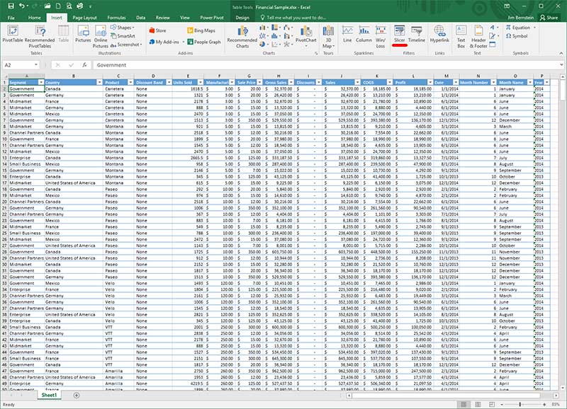
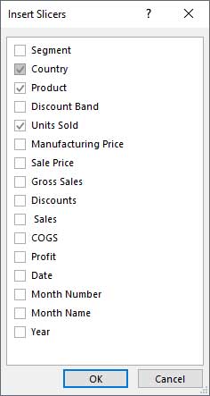
In our case we want to only see information about any number of units sold of the Paseo product in France. To do this simply click on the Slicers button and choose the categories from the list that you want displayed. So here we check the boxes for Country, Product and Units Sold since that’s the data we are looking for.
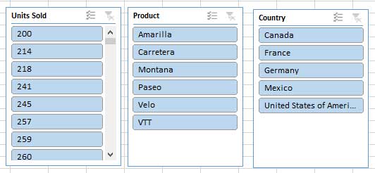
Once we click OK we are presented with a box for each of the “slices” we chose and it shows all of the possible values we have from those columns.
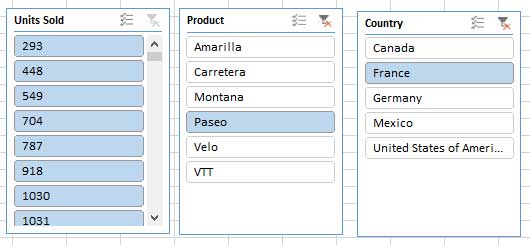
Next we will filter on any value for units sold but for the product called Paseo that have been sold in France by highlighting only what we want to show by clicking on the ones we don’t want to show so they are white. This will filter the sheet to only show these values under Country, Product and Units Sold that were selected.
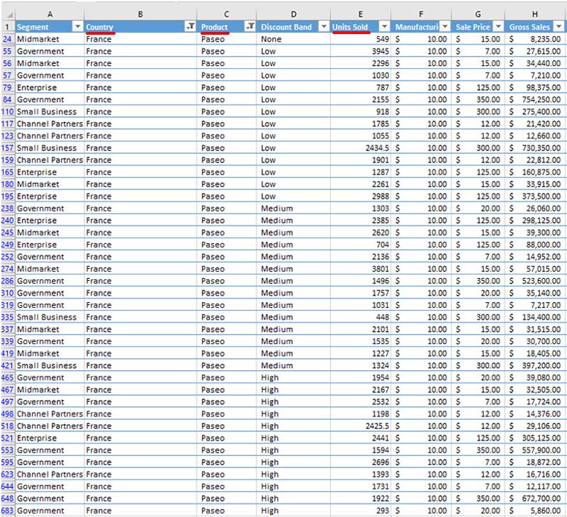
As you can see in our results the sheet is filtered by any unit amount sold of the product called Paseo that was sold in France. We have cut off part of the sheet to make things easier to see and all of the columns will still be displayed but only the data we filtered on will be shown.
Once you create your Slices you can click on or off whichever values you choose to filter your data. It’s a really efficient way to see only the data you want and at the same time have the ability to change your filters around as you need to. Using Slicers does not affect or remove any of your data so when it disappears don’t worry about it because it’s all still there. You can click on values to toggle them on and off and the results will update instantly. If you want to clear the filter for a particular slice then just click on the Clear Filter button on the top right. To remove a category all you need to do is right click on the slice you want gone and choose Remove “slice name” and it will disappear. Just be sure to clear the filter before doing so otherwise the data will remain filtered.


