
If you are a serious Excel user and have huge spreadsheets with a lot of data in them then managing your data can be a real task. If you need to worry about not having duplicate information in your spreadsheet then you can be in for some real time consuming work if you have to find duplicate values manually.
As datasets grow, even small inconsistencies can quietly undermine accuracy, reporting, and decision‑making. Duplicate entries may not always be obvious at a glance, yet they can distort totals, skew analysis, and create confusion when data is shared across teams. Having a reliable way to surface and address these issues early can save hours of cleanup later and help maintain confidence in the data you rely on every day.
For those who use Excel to store multiple entries in the same columns you may have wanted to be able to remove duplicates in your columns without having to sort through them manually.
Manually reviewing long columns row by row is not only inefficient, it also increases the risk of human error. When similar values appear scattered throughout a worksheet, duplicates can easily be overlooked or removed inconsistently. This is where built‑in Excel tools become especially valuable, allowing you to identify patterns and problem areas quickly without altering the underlying data structure.
Excel makes that easy by allowing to format the cells using a conditional format which will highlight the duplicate cells so you can remove the duplicates. It can also be used to highlight unique values. Be aware that you cannot conditionally format fields in the Values area of a PivotTable report by unique or duplicate values.

Here are the steps to highlight your duplicate cells:
1. Select one or more cells in your table.
2. On the Home tab, in the Style section, click the down arrow next to Conditional Formatting, and click Highlight Cells Rules.
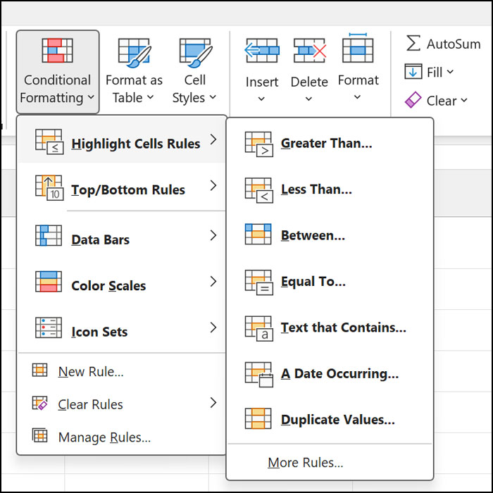
3. Select Duplicate Values from the list.
4. Choose the values that you want to use, either duplicate or unique and then select a format.
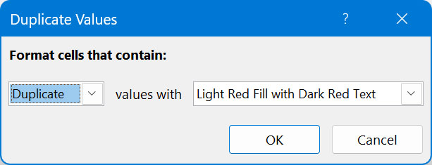
Now all the duplicate cells will be highlighted with the color you chose in step 4 making it easy to find and remove them.
In summary, Excel’s conditional formatting tools provide a fast, reliable way to identify duplicate and unique values without disrupting your data. By visually flagging potential issues, you can maintain cleaner spreadsheets, reduce errors, and spend less time on manual reviews. This approach not only improves efficiency but also helps ensure that your data remains accurate and trustworthy as your worksheets continue to grow.